📢 Introducing the Super-Resolution Validator for Segmentation Tasks
Benchmark your SR models in real-world segmentation workflows
In the world of Earth observation and computer vision, super-resolution models have come a long way in generating visually stunning and spatially enhanced outputs. But a critical question still lingers: Do they actually help when it matters? Specifically, do they improve downstream tasks like object segmentation?
Today, we’re excited to introduce a new tool that finally gives you a concrete way to answer that question:
✅ The Super-Resolution Model Validator
A lightweight, flexible validation framework to benchmark segmentation performance across Low-Resolution (LR), High-Resolution (HR), and Super-Resolved (SR) imagery — all with standardized and object-aware metrics.
🎯 Why We Built This
Most super-resolution research focuses on perceptual quality, PSNR, or visual inspection. But in applied domains like remote sensing, urban monitoring, or precision agriculture, what matters is task performance — like identifying buildings, roads, or trees.
That’s where this tool comes in. It lets you plug in segmentation models for LR, SR, and HR data and compare their performance side-by-side. You’ll see where your SR model helps (or doesn’t), and how much closer it brings your results to those achieved on native HR imagery.
🧪 What It Does
At its core, the validator performs controlled experiments across three image resolutions:
Low-Resolution (LR): The base input resolution (e.g., Sentinel-2 native)
Super-Resolved (SR): Output of your SR model
High-Resolution (HR): The “ground truth” benchmark (e.g., NAIP or manually annotated high-res imagery)
You run the same segmentation model (or a model adapted to each resolution) across each input type. The tool then:
Runs inference and caches results
Computes standard segmentation metrics (IoU, Dice, Precision, Recall, Accuracy)
Computes object-centric metrics, like:
Percentage of objects correctly identified
Accuracy split by object size
Average per-object prediction confidence
Outputs easy-to-read performance tables and mAP-style plots for visual inspection
🔍 Why This Matters
This tool isn’t just for scoring — it’s for understanding.
It helps you answer key questions:
Does my SR model really help segmentation?
How close is SR performance to the HR upper bound?
Are small objects more detectable after SR?
Is my model hallucinating texture, or recovering useful signal?
By explicitly comparing SR results to both LR and HR baselines, you gain a more scientific and honest view of what your SR pipeline is actually doing.
🚀 Getting Started
You can get started with just a few lines of code.
pip install opensr-usecases
Define your dataloaders and models (or use the built-in placeholders), then use the Validator class to run predictions, compute metrics, and visualize results.
Here’s a minimal example:
					# 0. Imports ------------------
from torch.utils.data import DataLoader
from tqdm import tqdm
from opensr_usecases import Validator


# 1. Get Data
# 1.1 Get Datasets
from opensr_usecases.data.placeholder_dataset import PlaceholderDataset
dataset_lr = PlaceholderDataset(phase="test", image_type="lr")
dataset_hr = PlaceholderDataset(phase="test", image_type="hr")
dataset_sr = PlaceholderDataset(phase="test", image_type="sr")

# 1.2 Create DataLoaders
dataloader_lr = DataLoader(dataset_lr, batch_size=4, shuffle=True)
dataloader_hr = DataLoader(dataset_hr, batch_size=4, shuffle=True)
dataloader_sr = DataLoader(dataset_sr, batch_size=4, shuffle=True)


# 2. Get Models ------------------
from opensr_usecases.models.placeholder_model import PlaceholderModel
lr_model = PlaceholderModel()
hr_model = PlaceholderModel()
sr_model = PlaceholderModel()


# 3. Validate ------------------
# 3.1 Create Validator object
val_obj = Validator(output_folder="data_folder", device="cpu", force_recalc= False, debugging=True)

# 3.2  Calculate images and save to Disk
val_obj.run_predictions(dataloader_lr, lr_model, pred_type="LR", load_pkl=True)
val_obj.run_predictions(dataloader_hr, hr_model, pred_type="HR", load_pkl=True)
val_obj.run_predictions(dataloader_sr, sr_model, pred_type="SR", load_pkl=True)

# 3.3 - Calcuate Metrics
# 3.3.1 Calculate Segmentation Metrics based on predictions
val_obj.calculate_segmentation_metrics(pred_type="LR", threshold=0.75)
val_obj.calculate_segmentation_metrics(pred_type="HR", threshold=0.75)
val_obj.calculate_segmentation_metrics(pred_type="SR", threshold=0.75)

# 3.3.2 Calculate Object Detection Metrics based on predictions
val_obj.calculate_object_detection_metrics(pred_type="LR", threshold=0.50)
val_obj.calculate_object_detection_metrics(pred_type="HR", threshold=0.50)
val_obj.calculate_object_detection_metrics(pred_type="SR", threshold=0.50)


# 4. Check out Results and Metrics ------------------
# 4.1 Visual Inspection
val_obj.save_results_examples(num_examples=1)

# 4.2 Check Segmentation Metrics
val_obj.print_segmentation_metrics(save_csv=True)
val_obj.print_segmentation_improvements(save_csv=True)

# 4.3 Check Object Detection Metrics
val_obj.print_object_detection_metrics(save_csv=True)
val_obj.print_object_detection_improvements(save_csv=True)

# 4.4 Check Threshold Curves
val_obj.plot_threshold_curves(metric="all")
📊 Output & Interpretation
The validator outputs:
Delta tables showing improvement from LR → SR, and gap to HR
mAP-style curves for object detection across thresholds
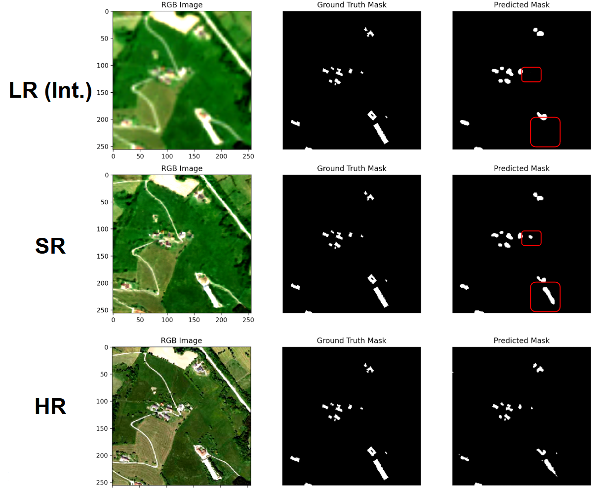
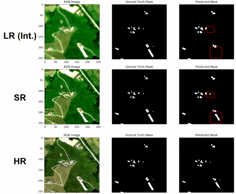
Side-by-side visualizations of ground truth, prediction, and uncertainty
CSVs and plots for easy reporting or publication
Example improvement table:
					+-----------------+----------+----------+-----------+----------+----------+
| Prediction Type |   IoU    |   Dice   | Precision |  Recall  | Accuracy |
+-----------------+----------+----------+-----------+----------+----------+
|        LR       | 0.091544 | 0.126083 |   0.1074  | 0.17869  | 0.974478 |
|        HR       | 0.147978 | 0.181809 |  0.172987 | 0.210582 | 0.986871 |
|        SR       | 0.085455 | 0.118916 |  0.104997 | 0.163465 | 0.974267 |
+-----------------+----------+----------+-----------+----------+----------+
+-----------+-----------+----------+-----------+
|   Metric  | LR → SR Δ |    SR    | HR → SR Δ |
+-----------+-----------+----------+-----------+
|    IoU    |  0.006089 | 0.085455 |  0.062523 |
|    Dice   |  0.007168 | 0.118916 |  0.062894 |
| Precision |  0.002403 | 0.104997 |  0.06799  |
|   Recall  |  0.015226 | 0.163465 |  0.047118 |
|  Accuracy |  0.000212 | 0.974267 |  0.012604 |
+-----------+-----------+----------+-----------+
+-----------------+---------------------------------+----------------------------+
| Prediction Type | Average Object Prediction Score | Percent of Buildings Found |
+-----------------+---------------------------------+----------------------------+
|        LR       |             0.465557            |          51.74534          |
|        HR       |             0.674343            |         72.931697          |
|        SR       |             0.441469            |         49.009067          |
+-----------------+---------------------------------+----------------------------+
+---------------------------------+-----------+-----------+-----------+
|              Metric             | LR → SR Δ |     SR    | HR → SR Δ |
+---------------------------------+-----------+-----------+-----------+
| Average Object Prediction Score |  0.024088 |  0.441469 |  0.232874 |
|    Percent of Buildings Found   |  2.736274 | 49.009067 |  23.92263 |
+---------------------------------+-----------+-----------+-----------+
💬 Final Thoughts
It’s easy to be impressed by pretty SR images. But in practice, those images need to work. This validator gives you a way to prove — or disprove — that your SR pipeline actually helps.
Whether you’re publishing a new model, building a remote sensing application, or refining your training data, this tool helps you close the loop between SR fidelity and task performance.
Give it a try, and if you like it, star the repo or contribute!
📦 opensr-usecases on GitHub