We’re excited to share the release of SEN2NAIP v2.0, a powerful and extensive dataset developed to support super-resolution (SR) research for Sentinel-2 imagery. Designed by our team and now hosted on Hugging Face, SEN2NAIP provides the foundation for both reference-based SR and synthetic training setups, enabling robust benchmarking and model development across varied spatial and spectral domains.
What’s Inside SEN2NAIP v2.0?
The dataset consists of two core components:
Cross-Sensor Dataset
2,851 image pairs pairing Sentinel-2 L2A imagery (low-resolution) with high-resolution NAIP orthophotos.
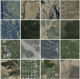
Each pair covers ~1.46 km², offering rich variability across landscape types.
Ideal for training and validating SR models in real-world remote sensing tasks.
Synthetic Dataset
17,657+ NAIP-S2like pairs, created by applying a trained degradation model that simulates Sentinel-2 characteristics from NAIP imagery.
Multiple variants using VAE and gamma-based histogram matching allow for comprehensive SR evaluation under different degradation assumptions.
The dataset also includes temporal support, cloud-optimized access, and updated harmonization models. You can explore and download it here on Hugging Face or use the ready-to-run Colab examples.
Why It Matters
SEN2NAIP addresses a critical bottleneck in SR research: the lack of realistic, high-quality, and diverse training data for satellite image enhancement. By bridging real and synthetic data pipelines with a unified framework, the dataset enables the development of robust SR models that generalize well across geographies, seasons, and sensors.
Whether you’re developing GANs, diffusion-based SR pipelines, or transformer-based upscaling networks, SEN2NAIP offers the benchmark data you need.
Dataset Usage Example
import matplotlib.pyplot as plt
import numpy as np
import tacoreader
# Load the dataset
dataset = tacoreader.load("tacofoundation:sen2naipv2-unet")
# Filter the dataset for a subset of classes in "rai:admin2"
top_classes = dataset["rai:admin1"].value_counts().index[:10] # Select top 5 most frequent classes
filtered_dataset = dataset[dataset["rai:admin1"].isin(top_classes)]
# Create subplots
fig, axes = plt.subplots(2, 2, figsize=(16, 12))
# Plot "rai:ele" (elevation)
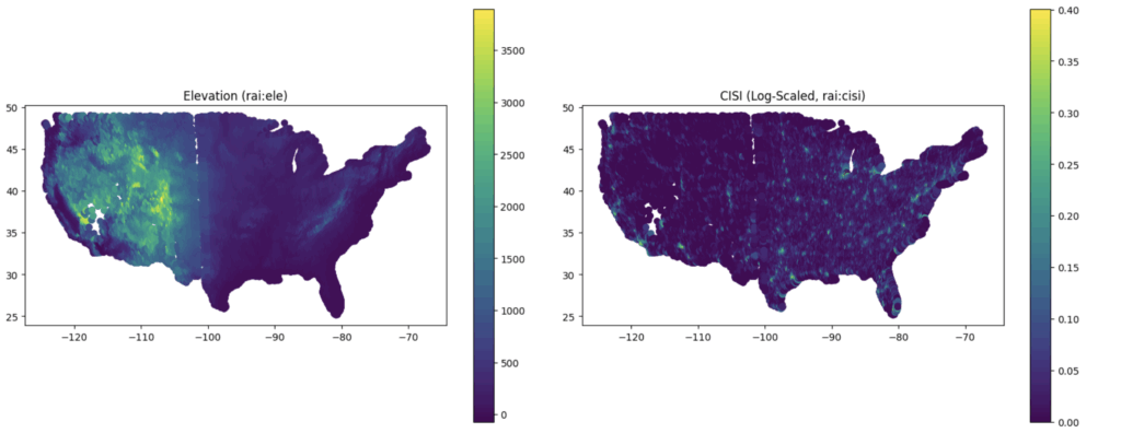
dataset.plot("rai:ele", cmap="viridis", legend=True, ax=axes[0, 0])
axes[0, 0].set_title("Elevation (rai:ele)")
# Plot "rai:cisi" (log-scaled) on the fly
dataset.assign(rai_cisi_log=lambda df: np.log1p(df["rai:cisi"])).plot(
"rai_cisi_log", cmap="viridis", legend=True, ax=axes[0, 1]
)
axes[0, 1].set_title("CISI (Log-Scaled, rai:cisi)")
# Plot "rai:admin0" (categorical) with a categorical colormap
dataset.plot("rai:admin0", cmap="tab20", legend=True, ax=axes[1, 0])
axes[1, 0].set_title("Administrative Boundaries (Level 0) (rai:admin0)")
# Plot filtered "rai:admin2" (categorical) with a limited number of classes
filtered_dataset.plot("rai:admin1", cmap="tab20", legend=True, ax=axes[1, 1])
axes[1, 1].set_title("Administrative Boundaries (Level 1, Filtered) (rai:admin1)")
# Adjust layout for better readability
plt.tight_layout()
plt.show()